Modeling the Fermentation
This page describes a set of models we built to turn the more than 10,000 measurements from around 50 different fermentations into something more useful: a compact mathematical fingerprint of how each fermentation unfolded.
The Basics
When the grape must reaches the fermentation tank, a two- to three-week scramble begins. Yeast converts sugar into alcohol; color and tannin migrate out of the skins and seeds into the juice; and the acid balance shifts. We follow all of this with a spectrometer and a handful of bench measurements, sampling each fermenting batch every day or two. The result is a thicket of numbers — for a single ferment, a dozen quantities each measured a dozen or more times.
The model's job is to replace that thicket, for each quantity, with one smooth curve and a few numbers that describe it: when color peaked, how fast the sugar fell, how much tannin we ended up with. Once every fermentation is summarized in the same way, we can compare vintages on an equal footing, flag a batch that is behaving oddly while we can still do something about it, and — eventually — predict where a ferment is heading from its first few days. We call these curves trajectories, and the collection of them a kinetic model — kinetic because it is about rates, about how fast things happen.
What We Measure
For each fermentation batch we track ten quantities. In plain terms:
Sugar (°Brix) — the food supply, falling as the yeast consume it.
Alcohol — rising as the sugar disappears.
Free, bound, and total anthocyanins — the red pigments.
Tannins and total iron-reactive phenolics — structure and mouthfeel.
Titratable acidity and pH — the acid balance.
Volatile acidity — the faint whiff of vinegar we hope stays low.
We also record the temperature at every sampling, which turns out to matter more than anything else (see below). All told, the years from the late-1990s to today add up to 49 fermentations and just under a thousand individual measurements consistently gathered.
The Right Clock: Temperature-Adjusted Time
Here is the single most important idea on this page. Chemistry runs faster at elevated temperatures. A day of cold soak at 50 dF barely moves the needle; a day of vigorous fermentation at an excessive 95 dF accomplishes a great deal. So calendar time — days since harvest — is the wrong yardstick for how far a ferment has progressed. Two batches that are three days in can be in entirely different places if one was kept cold and the other warm. That temperature governs extraction is well established in the winemaking literature [2, 3, 5].
Figure 1. (A) The chemistry runs faster when it is warm: each observed temperature becomes a speed multiplier. A cold-soak day at 50 °F counts for about a tenth of a reference day; a warm fermentation day at 95 °F counts for five. (B) Adding those multipliers up gives “thermal time” τ. For this 2023 Cabernet the cold soak barely advances the clock, then warm primary fermentation races ahead of the calendar.
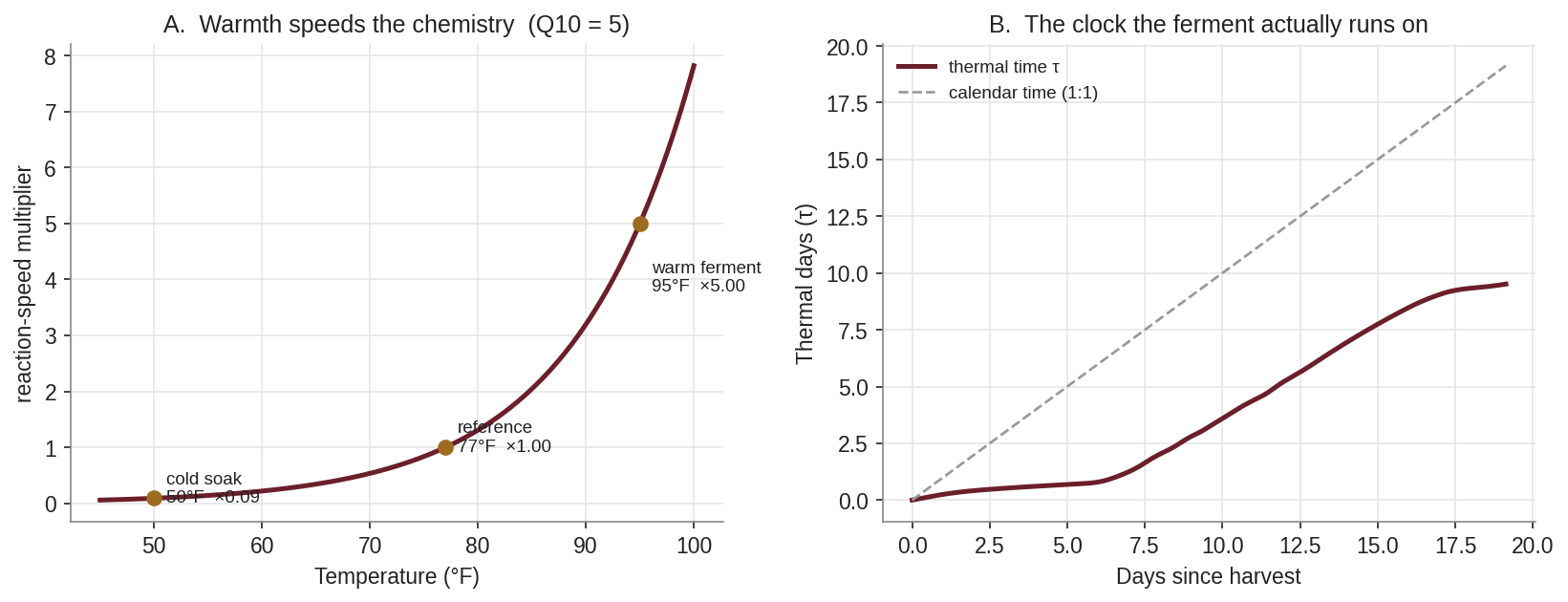
We fix this by stretching and compressing the clock according to temperature. Every observed temperature is turned into a speed multiplier:
f(T) = Q10 ^ ( (T − 77 °F) / 18 )
Three numbers set the scale: a reference temperature (77 dF, where the multiplier is exactly one), the 18 dF that corresponds to a 10 °C step (the rule is conventionally stated per 10 °C), and Q10 — the factor by which the rate rises for each such step. Summing these multipliers over the fermentation gives thermal time, written τ (“tau”). A warm day contributes several thermal days; a cold-soak day a fraction of one.
How temperature-sensitive is the chemistry — what is Q10? The textbook default is 2, meaning the rate doubles every 10 °C. We did not want to assume it, so we let our own data choose: we refit every batch across a range of Q10 values and asked which produced the cleanest curves.
Figure 2. Fit quality as the temperature-sensitivity Q10 is varied. Sugar and alcohol (the yeast's work) barely care. But color and tannin extraction clearly prefer a much steeper Q10 — around 5 — than the textbook value of 2
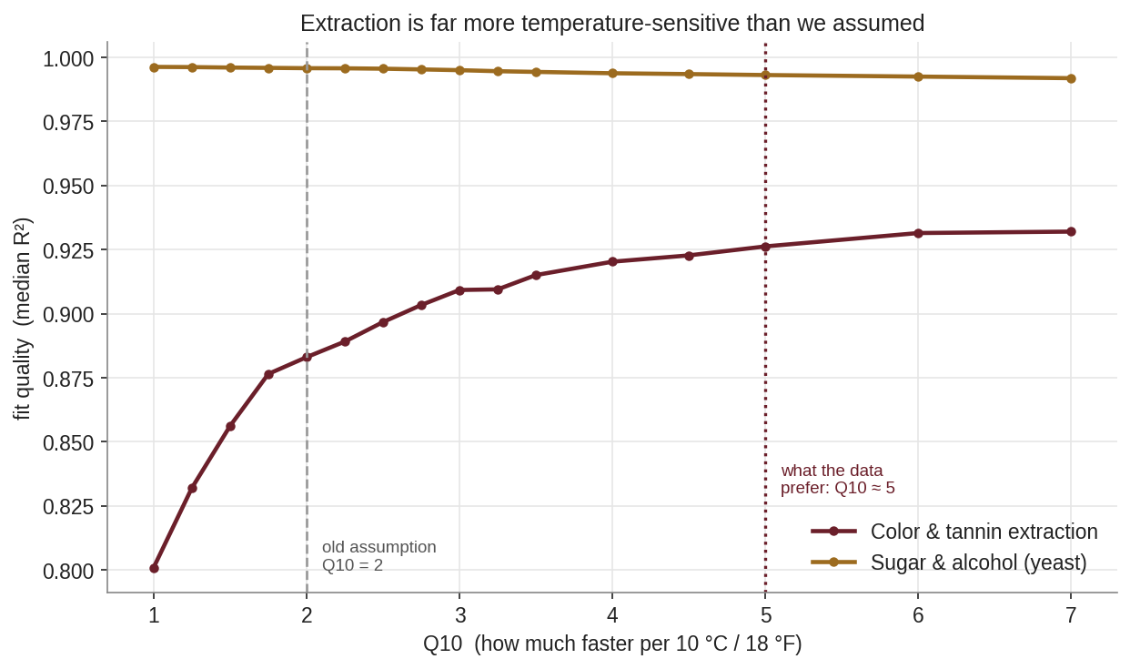
The answer surprised us. For sugar and alcohol — the yeast's work — Q10 hardly matters; those fits are excellent at any value. But for color and tannin extraction the data clearly prefer a far steeper Q10, around 5 to 7. Extraction roughly quintuples, rather than doubles, for each 10 °C. In hindsight this makes sense: pulling pigment and tannin out of the skins is not gentle diffusion but depends on the skin cells breaking down, which heat accelerates sharply — a temperature dependence that mechanistic extraction models capture through activation energies [5]. We settled on Q10 = 5 for everything; it captures almost all of the gain for extraction and costs nothing for the yeast variables. (Reassuringly, this preference for a steep Q10 is just as strong in batches that never saw a cold soak, so it is a genuine temperature effect.)
One Curve per Process: The Model Families
Figure 3. Four chemistry-matched curve shapes, each with only three or four parameters
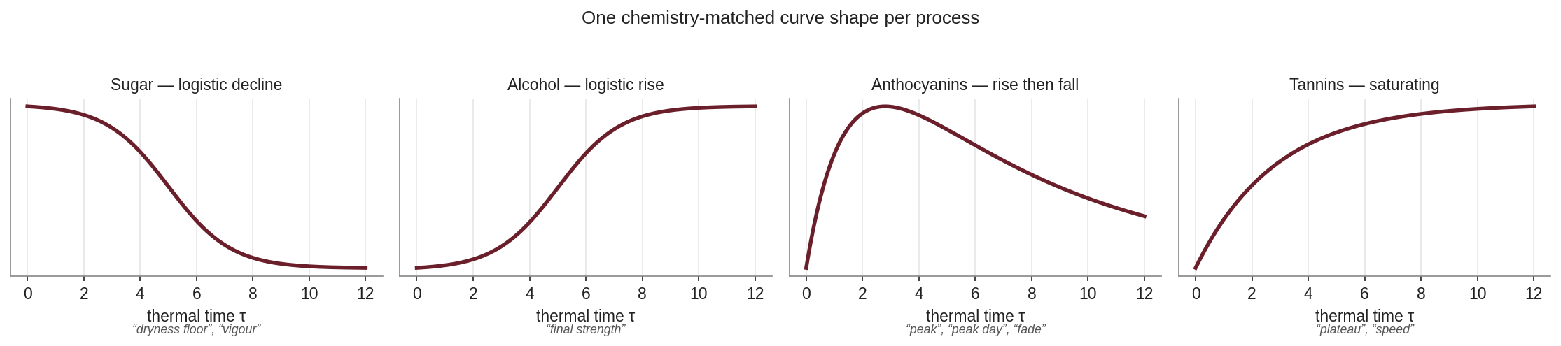
A good model curve should have the right shape for the chemistry it describes, with as few adjustable parameters as possible. We use four shapes, each with precedent in the food- and wine-science literature:
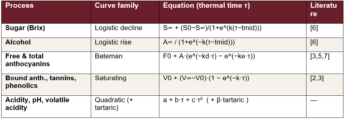
Logistic — the sugar curve falls in an S — slow at first while the yeast establish themselves, fast in the middle, slow again as the last sugar is consumed; alcohol is its mirror image, an S-shaped rise. The logistic form is a standard description of fermentation kinetics [6].
Bateman (rise then fall) — color is extracted quickly, peaks, then declines as pigment binds to other compounds or precipitates. This “appears, then disappears” behavior — extraction followed by reaction — is exactly what extraction studies report for anthocyanins [3, 5], and the classic mathematical shape for it is the Bateman curve [7]. It fits free and total anthocyanins.
Saturating — tannins and the other phenolics climb quickly and then level off at a plateau, the saturating shape seen for skin-derived phenolics during maceration [2, 3].
Quadratic — acidity, pH and volatile acidity drift gently and are well described by a simple parabola, whose turning point conveniently marks, say, the day acidity peaked.
Table 1. Curve family by process, with supporting literature (see References).
Reading the Parameters
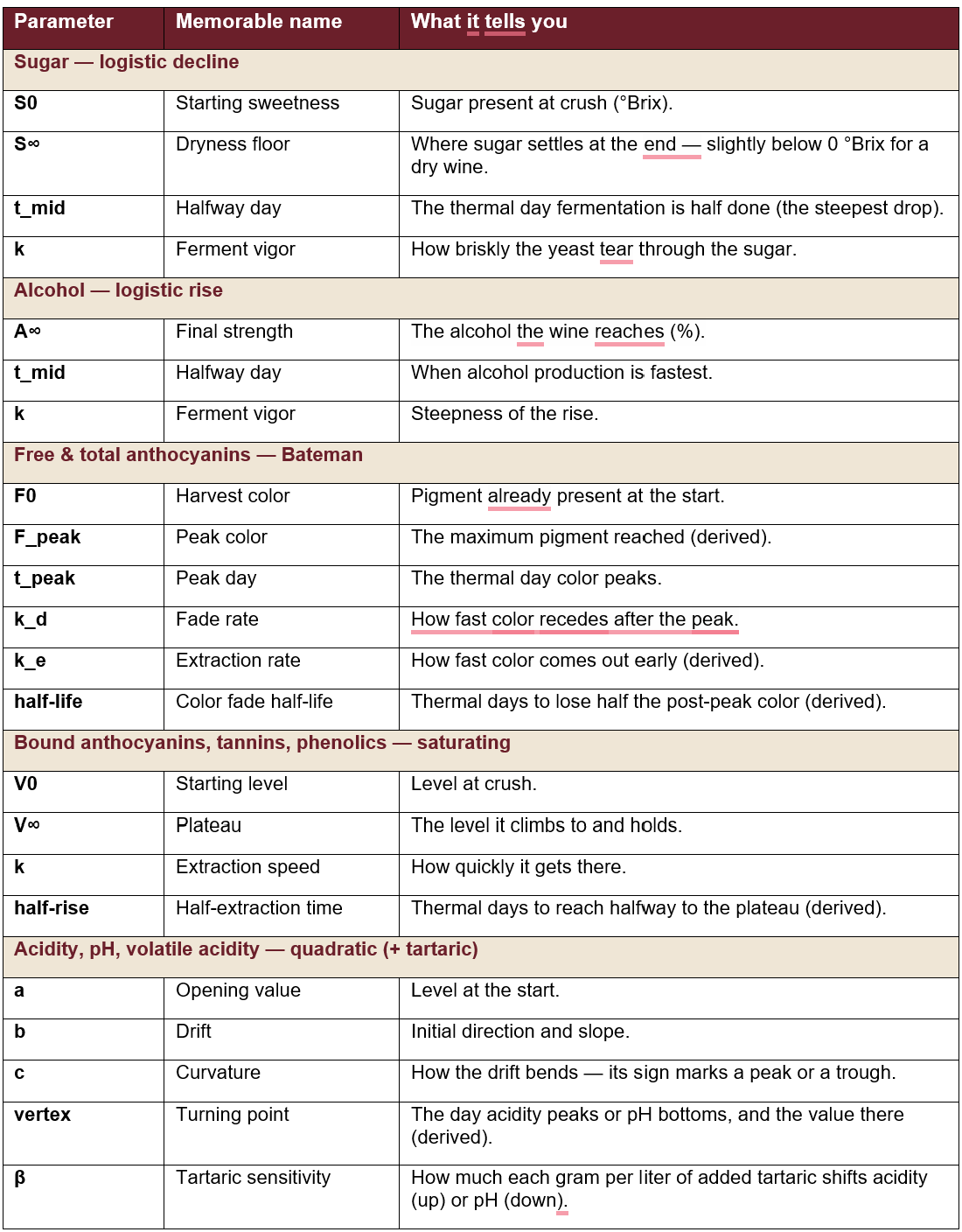
Each shape carries a handful of parameters — typically three or four — and those parameters are exactly the compact summary we were after. We have given each a plain-language name so the numbers mean something at a glance. Figure 4 shows them on a real color curve; Table 2 is the full dictionary.
Figure 4. The named parameters on the 2023 Cabernet free-anthocyanin (color) curve: harvest color, the peak and the day it occurs, and the half-life of the fade afterward
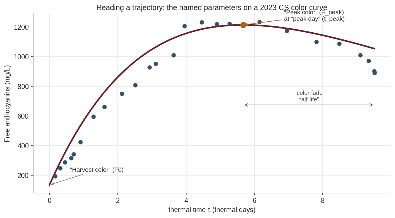
Table 2. The parameter dictionary — a plain-language name and meaning for every parameter
Fitting the Curves - A Fermentation Fingerprint
Figure 5. All ten trajectories for the 2023 Cabernet Sauvignon, shown together — its fingerprint. Dots are measurements; lines are the fitted model. Sugar falls and alcohol rises in mirror-image S-curves; free and total anthocyanins rise to a peak and recede; tannins and phenolics climb to a plateau; acidity and pH drift.
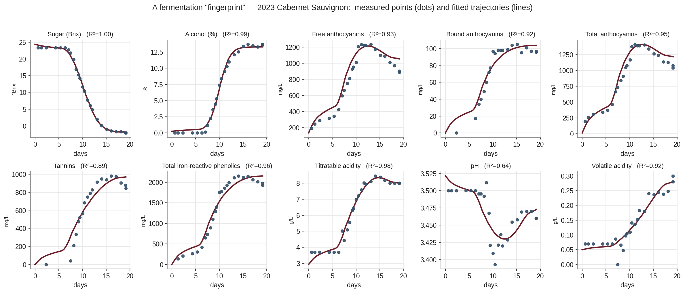
To fit a batch, we compute its thermal-time clock once, then find, for each quantity, the curve parameters that best match the measured points (ordinary least squares). The charts above show the curves against the observed values. This turns out to be a great way to spot outliers. We define outliers as data points that lie at least 3 mean square errors away from the curve and adjust those automatically to their curve fitted value. Then we rerun the curve fitting again and present an adjusted fingerprint. This auto-adjustment is done only once.
Table 3 gives the typical (median) agreement across all 49 ferments, reported as R² — the fraction of the variation the curve captures, where 1.00 is perfect.
Table 3. Typical fit quality, median R² across 49 fermentations
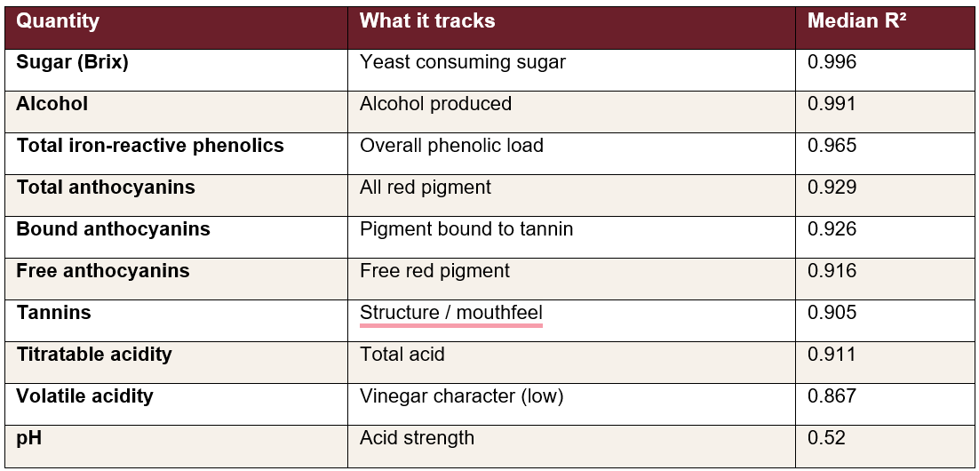
The yeast variables are essentially perfect, and the phenolics – the heart of red-wine quality – land between 0.90 and 0.97. The two quantities hardest to fit are volatile acidity, which is genuinely noisy at the tiny concentrations involved, and pH, which barely changes during fermentation and so offers little signal for any curve to grip. The one-time outlier adjustment lifts volatile acidity, but pH stays low – and a low R² there reflects a flat, quiet quantity, not a bad model.
The Fingerprint in Numbers
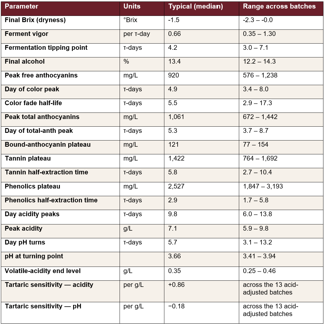
Put together, about twenty parameters define a fermentation's fingerprint. The table below lists them with a typical value (the median across all our ferments) and the range we actually see from batch to batch (the 10th to 90th percentile). Times are in thermal days (τ). This is, in a sense, the whole point of the exercise: the entire history of a fermentation, compressed into one comparable row of numbers.
Table 4. The ~20 parameters that define a fermentation fingerprint, with typical values and batch-to-batch range
Acidity and Adding Tartaric Acid
Figure 6. A 2017 Cabernet lot that received two tartaric additions (gold lines): titratable acidity jumps and pH dips at each addition. The model takes our additions as an explicit input and follows along, keeping the natural drift and the deliberate additions separate.
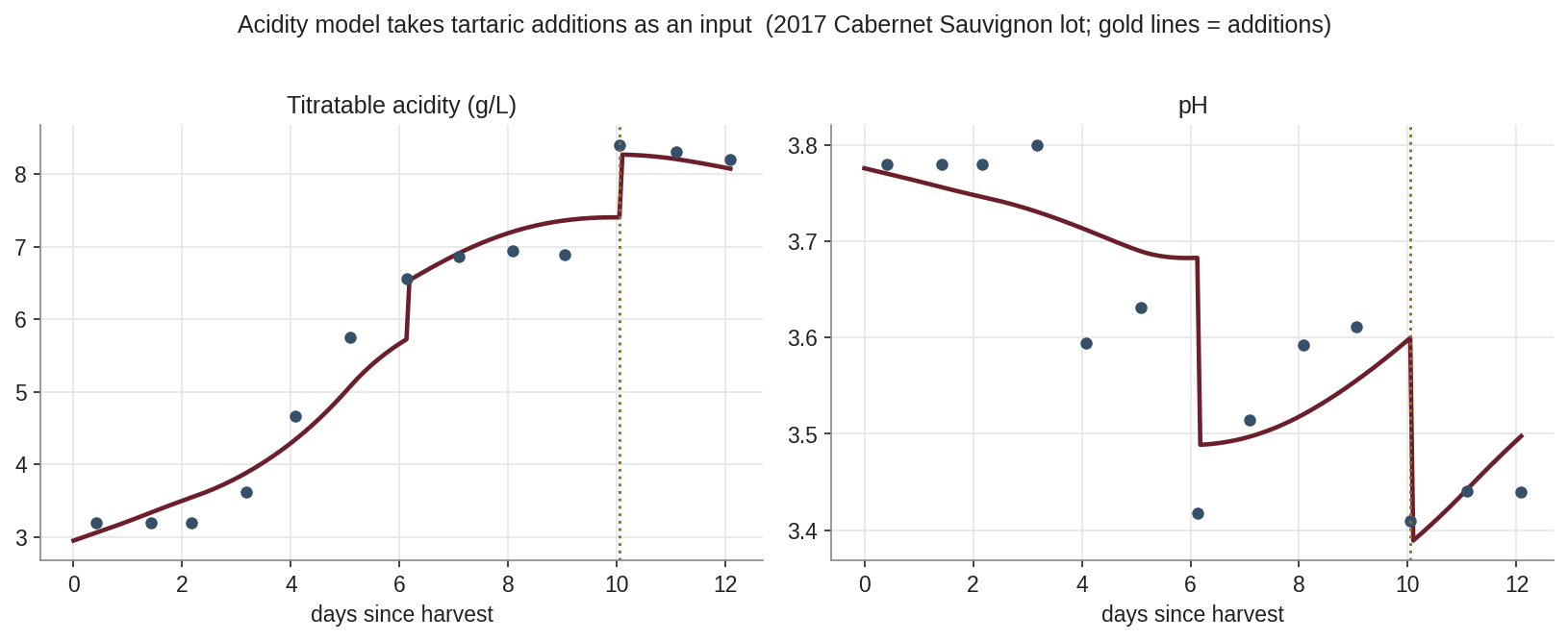
Acidity carries one complication the other quantities do not: we sometimes add tartaric acid to the must. An addition is not chemistry the ferment did on its own — it is something we did to it — and it appears as a step up in titratable acidity and a step down in pH. Pretending those steps are part of a smooth, natural trajectory would be wrong, so for pH and acidity the model takes our additions as an explicit input. We record the cumulative tartaric added, and the curve becomes “the natural trajectory plus the effect of what we poured in.” Our own data say each gram per liter of tartaric raises titratable acidity by about 0.86 g/L (close to the textbook stoichiometric expectation) and lowers pH by about 0.18 — figures that hold steady from batch to batch.
We will admit the obvious: we have on occasion overdone the tartaric — the 2015 vintage remains the cautionary tale — and being able to see additions cleanly separated from the natural acid drift is exactly the sort of hindsight this whole exercise is meant to give us.
A Family Portrait of the Vintages
Once every fermentation is reduced to the same handful of numbers, a natural question follows: do our ferments fall into families? To find out, we placed all 47 fermentations in the space of their fingerprint parameters and used a standard technique – principal component analysis – to collapse those 17 numbers into the two directions along which the fermentations differ most. Each dot below is one fermentation; ferments that sit close together behave alike.
The horizontal axis turns out to track extraction intensity – how much color and tannin came out of the skins, increasing to the right. The vertical axis tracks pace – fast, early-peaking ferments toward the top, and slow, late-peaking toward the bottom. Together, these two directions capture about 40% of the variation; the fingerprint is genuinely many-sided, so this is a flattened shadow of a higher-dimensional cloud, not the whole truth.
Figure 7: Each point is one fermentation, placed by its fingerprint. Left: colored by grape variety, with shaded 1.8-σ regions – Cabernet Sauvignon and Merlot overlap almost entirely. Right: the families the data themselves suggest, including a distinct Petit-Verdot / Cabernet-Franc blend group on the high-extraction side.
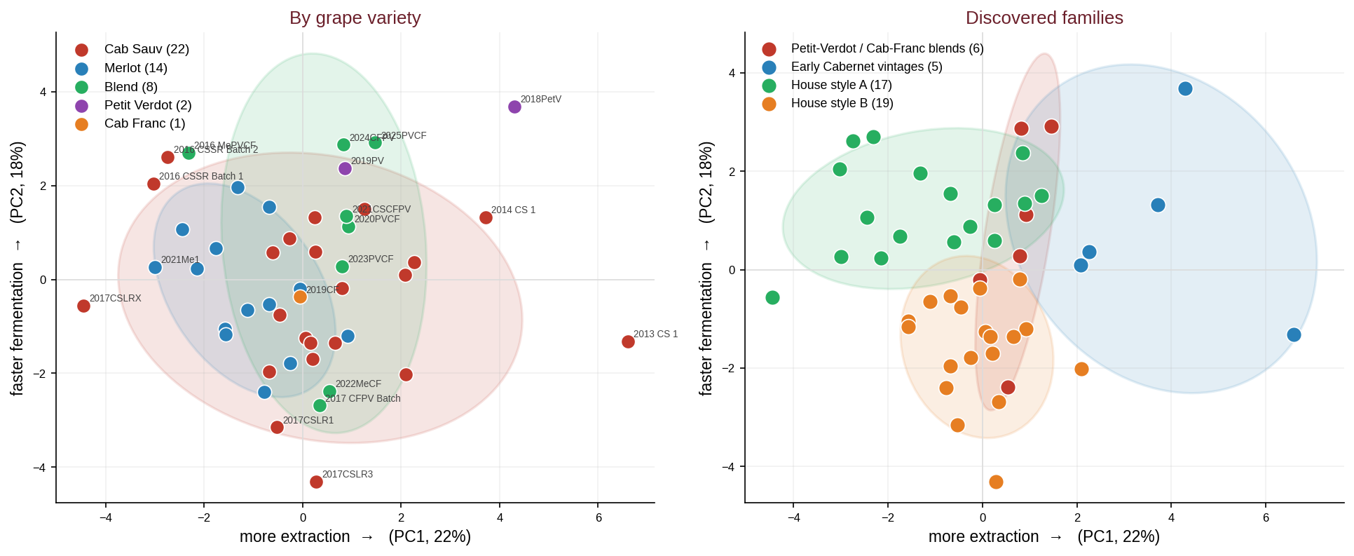
Two things stand out. First, grape variety is not the dividing line one might expect: our Cabernet Sauvignon and Merlot ferments overlap almost completely – the red and blue regions sit one on top of the other. How a batch ferments – how fast, and how much it extracts – depends more on the vintage and on what we did in the cellar than on which grape was in the tank. Second, one family genuinely keeps to itself: the Petit-Verdot and Cabernet-Franc blends cluster together on the high-extraction side, a recognizably distinct style. A small group of our earliest Cabernet vintages also sits apart – a reminder of how much our methods have changed since 2013.
We do not read too much into the exact boundaries – fifty fermentations is a modest sample – but as a family portrait, it already earns its keep: it shows which ferments are typical, which are unusual, and where a new vintage will fall relative to its predecessors. Whether these families also track the wines we end up enjoying most is a question we are keeping for a later page.
What We Have Learned — and What We Have Not
Temperature is the master variable. The biggest single improvement in the whole exercise came not from a cleverer curve but from using the right clock — and from discovering that extraction is far more heat-sensitive than the textbook number suggests.
A fermentation can be summarized compactly. Every ferment, past and future, reduces to a comparable fingerprint of about twenty numbers. This fingerprint also allows for the identification and auto-adjustment of outliers in the underlying data
Some things resist modeling. pH is nearly flat, volatile acidity is noisy, and the gentle parabolas we use for acidity describe the observed window well but should not be trusted to extrapolate beyond it. We would rather state these limits than paper over them.
Where This Goes Next
With a consistent fingerprint for every vintage, we can begin to ask better questions. Which ferments were unusually slow, and did it show in the glass years later? Can the first three days predict the peak? How do the same grapes behave in a warm year versus a cool one, once temperature is accounted for? Those are the threads we will pull on in the rest of this Analytics section.
References
[1] Boulton, R. B., Singleton, V. L., Bisson, L. F., & Kunkee, R. E. (1996). Principles and Practices of Winemaking. New York: Springer.
[2] Sacchi, K. L., Bisson, L. F., & Adams, D. O. (2005). A review of the effect of winemaking techniques on phenolic extraction in red wines. American Journal of Enology and Viticulture, 56(3), 197–206.
[3] Setford, P. C., Jeffery, D. W., Grbin, P. R., & Muhlack, R. A. (2017). Factors affecting extraction and evolution of phenolic compounds during red wine maceration and the role of process modelling. Trends in Food Science & Technology, 69, 106–117.
[4] Setford, P. C., Jeffery, D. W., Grbin, P. R., & Muhlack, R. A. (2019). Mathematical modelling of anthocyanin mass transfer to predict extraction in simulated red wine fermentation scenarios. Food Research International, 121, 705–713.
[5] Miller, K. V., Noguera, R., Beaver, J., Medina-Plaza, C., Oberholster, A., & Block, D. E. (2019). A mechanistic model for the extraction of phenolics from grapes during red wine fermentation. Molecules, 24(7), 1275.
[6] Wang, D., Xu, Y., Hu, J., & Zhao, G. (2004). Fermentation kinetics of different sugars by apple wine yeast Saccharomyces cerevisiae. Journal of the Institute of Brewing, 110(4), 340–346.
[7] Bateman, H. (1910). The solution of a system of differential equations occurring in the theory of radioactive transformations. Proceedings of the Cambridge Philosophical Society, 15, 423–427.
Last updated June 20, 2026