Spectra and Color Evolution

Since 2013, every must and wine we make has passed through a spectrometer – daily for each fermentation batch, monthly for each cellar batch. We have recorded full absorption spectra — 200 to 900 nanometers as a first step in estimating phenolic characteristics (see the page on Phenolics in Wine in the Laboratory section, http://chateauhetsakais.com/winexray-phenolics). This page describes how we turn those raw spectra into the color a person actually sees, the CIE L*a*b* coordinates, and what the resulting trajectories tell us about how a red wine builds its color in the tank and slowly transforms it in the barrel. This page is organized into 4 sections

Remove the noise in the recorded spectral data: the noise is mostly a consequence of calibrating the sample against water
Describe color with the CIE parameters
Look at the evolution of color in a single vintage (2014) from harvest through press to bottling
Compare the color evolution of the 5 cabernet sauvignon vintages (2014, 2017, 2018, 2019 & 2020)
This will lead us to a few paths to explore further.

Cleaning the recorded spectral data

Each record contains absorbance measurements taken at 1-nanometer intervals from 200 to 900 nm. Absorbance is a physical quantity that cannot be negative, yet roughly one reading in ten in our data sits slightly below zero. These negatives are not scattered at random: they cluster in the red and near-infrared region beyond about 650 nm, exactly where a red wine absorbs almost no light and the true signal is near zero. The dips are tiny — a median of about −0.001 absorbance units — and in the near-infrared they are centered on zero. That is the fingerprint of zero-mean random baseline noise from the instrument and its calibration, not a systematic offset.

The obvious fix — clipping every negative value up to zero — is the wrong one. Because the noise is symmetric about zero, rectifying it to one side introduces a systematic positive bias precisely in the low-signal red region, which would make every wine compute as slightly redder than it is. Instead, we apply a Savitzky–Golay smoothing filter (a second-order polynomial over an eleven-nanometer window) along the wavelength axis [3]. Smoothing preserves the local average while averaging away the high-frequency noise, removing the scatter without the bias that clipping introduces; any tiny residual negatives are then floored to zero. The negatives beyond 780 nm fall outside the visible range and never enter the color calculation [1, 2].

In a Savitzky–Golay filter each smoothed point is a fixed weighted average of the raw readings in a small window around it:

ŷ(i) = Σ c(j) · y(i+j), j = −5 … +5

The weights c(j) depend only on the window length and the polynomial order. For our choice — eleven points, second order — they are the coefficients that best fit a second-order polynomial to the window (±5 nm) in the least-squares sense, so the filter follows the genuine curvature of the spectrum while cancelling the point-to-point noise. The weights have a simple closed form, w(j) = (89 − 5·j²) ⁄ 429 for j = −5 … +5 — that is, [−36, 9, 44, 69, 84, 89, 84, 69, 44, 9, −36] ⁄ 429. They are symmetric, they sum to one (so a flat or sloping baseline passes through unchanged), and the two end weights are slightly negative, which is exactly what lets the filter smooth noise without flattening genuine absorption peaks.

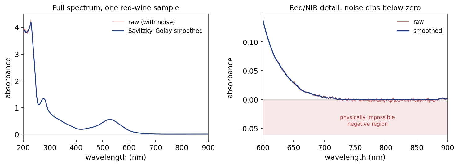
Figure 1. A representative red-wine spectrum. Left: the full 200–900 nm curve, dominated by the anthocyanin band near 520 nm; raw and smoothed traces coincide where signal is strong. Right: the red/near-infrared detail, where raw noise dips below zero into the physically impossible region and Savitzky–Golay smoothing recovers a clean, non-negative baseline.

From Spectrum to Color: The CIE Parameters

With the spectrum cleaned, absorbance is converted to transmittance using T = 10^(−A), the fraction of light transmitted by the wine at each wavelength. That transmittance curve is weighted by the CIE 1964 10° standard observer and the D65 daylight illuminant and integrated across the visible range of 380 to 780 nm, following the OIV convention for wine color [1, 2]. The result is the set of tristimulus values X, Y, Z, which transform into the CIE 1976 L*a*b* coordinates [1].

One practical detail is optical pathlength. The Beer–Lambert law states that absorbance grows in direct proportion to the concentration of the absorbing species and to the distance the light travels through the sample:

A = ε · c · d

where ε is the molar absorptivity, c is the concentration, and d is the optical path length (the width of the measuring cell). Because absorbance is strictly linear in d, a spectrum recorded in a cell of one pathlength converts to any other pathlength by a single multiplicative constant:

A(d₂) = (d₂ ⁄ d₁) · A(d₁)

We checked the whole chain against WineXRay’s CIELab readings for the same samples. The two agreed to within rounding once we applied a factor of five.

CIE L*a*b* pinpoints any color with three numbers, designed so that equal numerical steps appear as roughly equal differences to the eye. Two further quantities, chroma and hue angle, re-express the same point in the way people naturally describe color. In a red wine, these coordinates are governed mainly by the anthocyanin pigments and, as the wine ages, by the copigmented and polymeric forms they evolve into [4, 6].

Table 1. The CIE color parameters and what each one tells you.

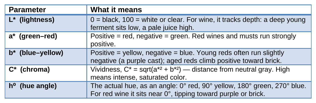
Note, C* and h⁰ carry no new information: they are simply the polar form of the Cartesian pair (a*, b*). A wine’s position on the green–red / blue–yellow plane can be named either by its coordinates (a*, b*) or, equivalently, by its distance from the neutral center and its angle around it:

C* = √(a*² + b*²) , h⁰ = atan2(b*, a*)

The mapping inverts exactly:

a* = C* · cos(h⁰) , b* = C* · sin(h⁰) .

Lightness L* is the independent third dimension. So a wine’s color is really two numbers plus a lightness; chroma and hue are just a more intuitive way of reading the same a*–b* point. The disk below illustrates the geometry.

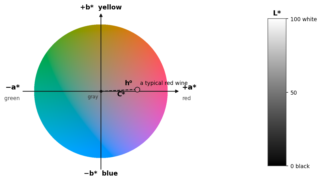
Figure 2. The CIE color space. The disk is the a*–b* plane at a fixed lightness: right is red (+a*), left green(-a*), up yellow (+b*), down blue (-b*). Hue h⁰ is the angle around the wheel, chroma C* the distance from the gray center, and the bar at right is lightness L*. A typical red wine sits just above the +a* axis at high chroma.

One Vintage in Detail: the 2014 Cabernet, as Measured

Following a single wine through its whole life makes the pattern concrete. The 2014 Cabernet was sampled daily during fermentation and then in barrel every few weeks to every couple of months across nearly three years of aging. In the graphic below, we plot each spectrum sample converted to color coordinates. On the a*–b* plane, the color traces a clear out-and-back loop. At crush, the juice is pale and sits near the neutral center; as anthocyanins extract from the skins, the point races outward along the red +a* axis and dips below it into negative b* — the bluish-purple of a young, heavily extracted red — reaching the rim near a* = 66 at peak color. The first triangle marks the low b* point, the second triangle, the high b* point, and the star marks the press. Over the following three years in barrel, the point drifts steadily inward, a* fading from about 61 toward 40, while b* edges up across zero from purple toward brick

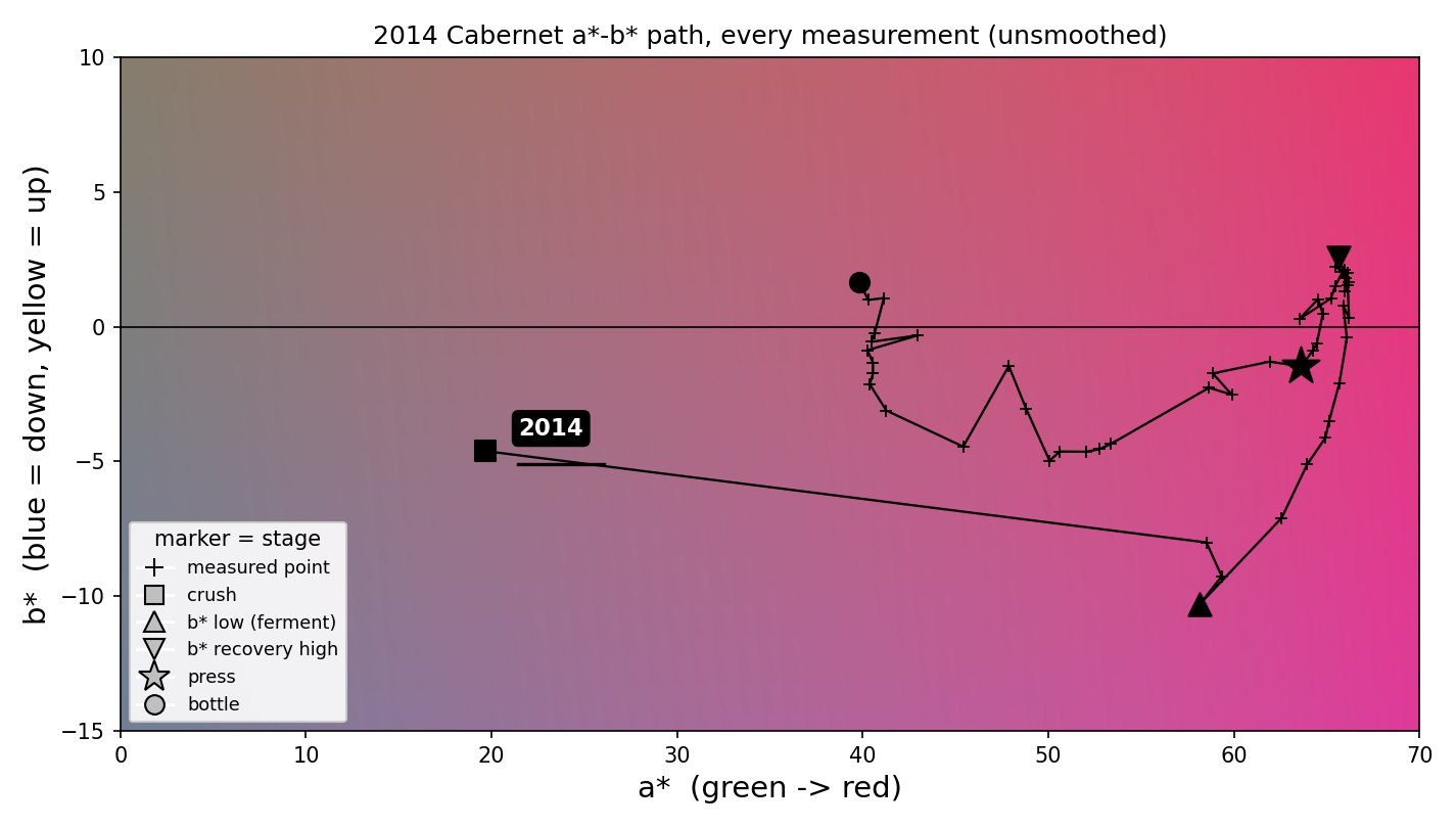
Figure 3. 2014 Cabernet a*-b* path, every measurement as recorded (unsmoothed). Crosses are individual measurements; the background shows the colour of each a*-b* point. Markers flag the stages: square = crush, up-triangle = the b* low during fermentation, down-triangle = its recovery, star = press, filled dot = bottle. Note how the barrel-aging points scatter from one sampling to the next.

Read as lightness over time, the same wine shows a steep plunge as color builds during fermentation, a dark floor before the press, and a gradual recovery as it clarifies in the cellar. Plotting time on a logarithmic axis lets the two weeks of fermentation and the years of cellaring share one frame. The cellar stretch is visibly noisy: successive samplings jump around by several lightness units, a mix of sampling variations in the barrel and ordinary measurement scatter.

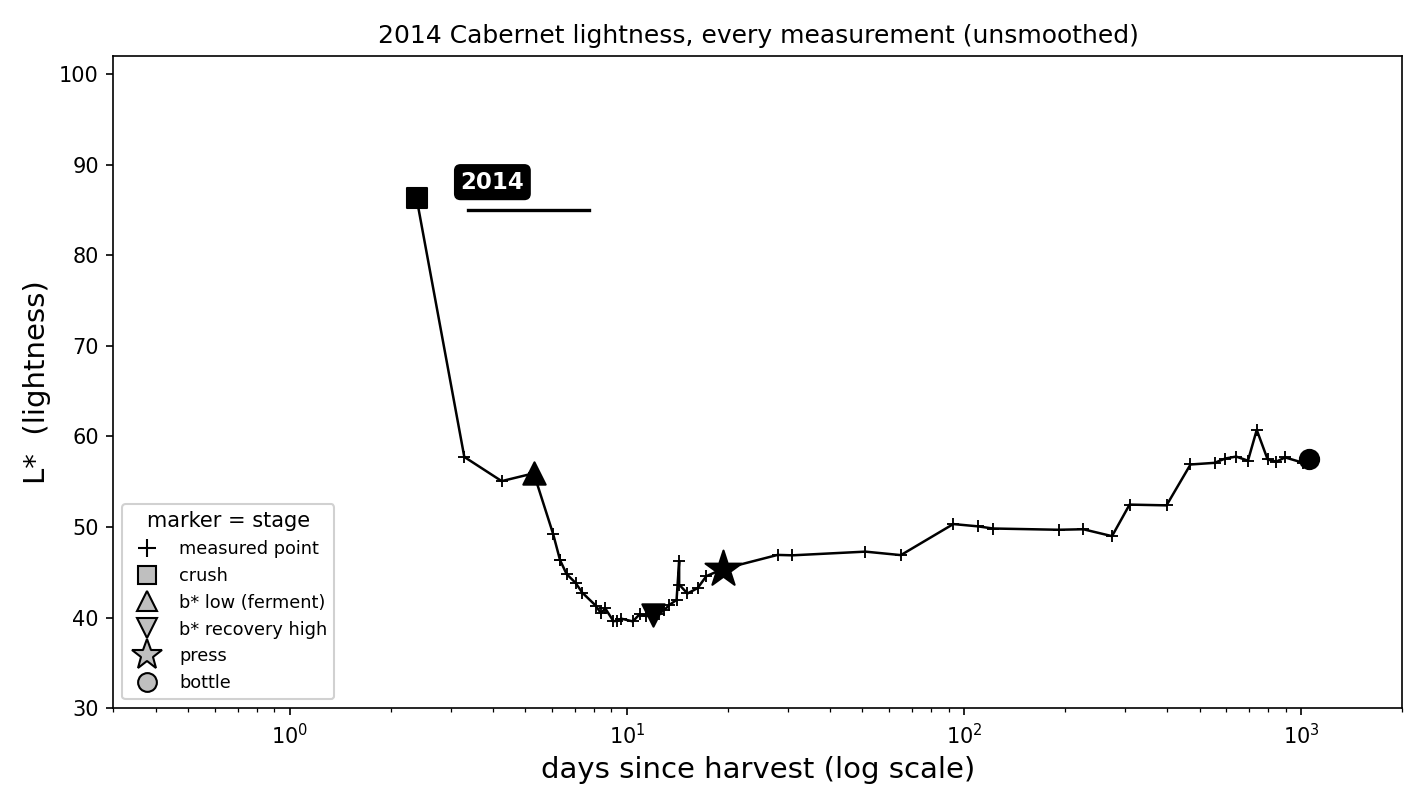
Figure 4. 2014 Cabernet lightness L* from crush to bottle on a logarithmic time axis, every cellar measurement shown. Lightness falls steeply during fermentation to a minimum near the press (star), then recovers gradually across nearly three years in barrel.

Smoothing the Trajectory

Both parts of the trajectory carry the same measurement noise, so we smooth both - but by different amounts, matched to how fast each part moves. The smoother is a time-weighted average (a Gaussian kernel in logarithmic time) that lets each point borrow strength from its neighbours in time. Fermentation is fast and densely sampled, so it needs only a light touch - a narrow kernel that follows the rapid out-and-back excursion while trimming the point-to-point jitter. Cellaring is the opposite: the wine changes slowly over years and each reading carries the same noise, so we smooth it more strongly with a wider kernel to recover the slow drift. This is deliberately not a fitted model - the trajectory follows no assumed equation, unlike the kinetic curves we fit to fermentation - it is simply a way to see the underlying path through the scatter. The figures below repeat the 2014 path smoothed, with the raw measurements kept visible as small crosses.

Concretely, the smoothed value at any time t is a weighted average of every cellar reading y(i) recorded at its own time t(i):

ŷ(t) = [ Σ w(t,i) · y(i) ] ⁄ [ Σ w(t,i) ] ,

w(t,i) = exp( −[ log₁₀ t − log₁₀ t(i) ]² ⁄ 2h² )

The weight w(t,i) is a Gaussian in the logarithm of time: a reading counts fully when it is close in log-time to t and fades smoothly as it moves away, with the bandwidth h setting how strongly neighbouring points are blended. We use a narrow h of about 0.08 decades for the fast fermentation and a wider h of about 0.16 decades (roughly a factor of 1.4 in age) for the slow cellar aging. Working in log-time matches the logarithmic time axis of the plots and keeps the early, closely spaced samplings from being overwhelmed by the long tail of later ones.

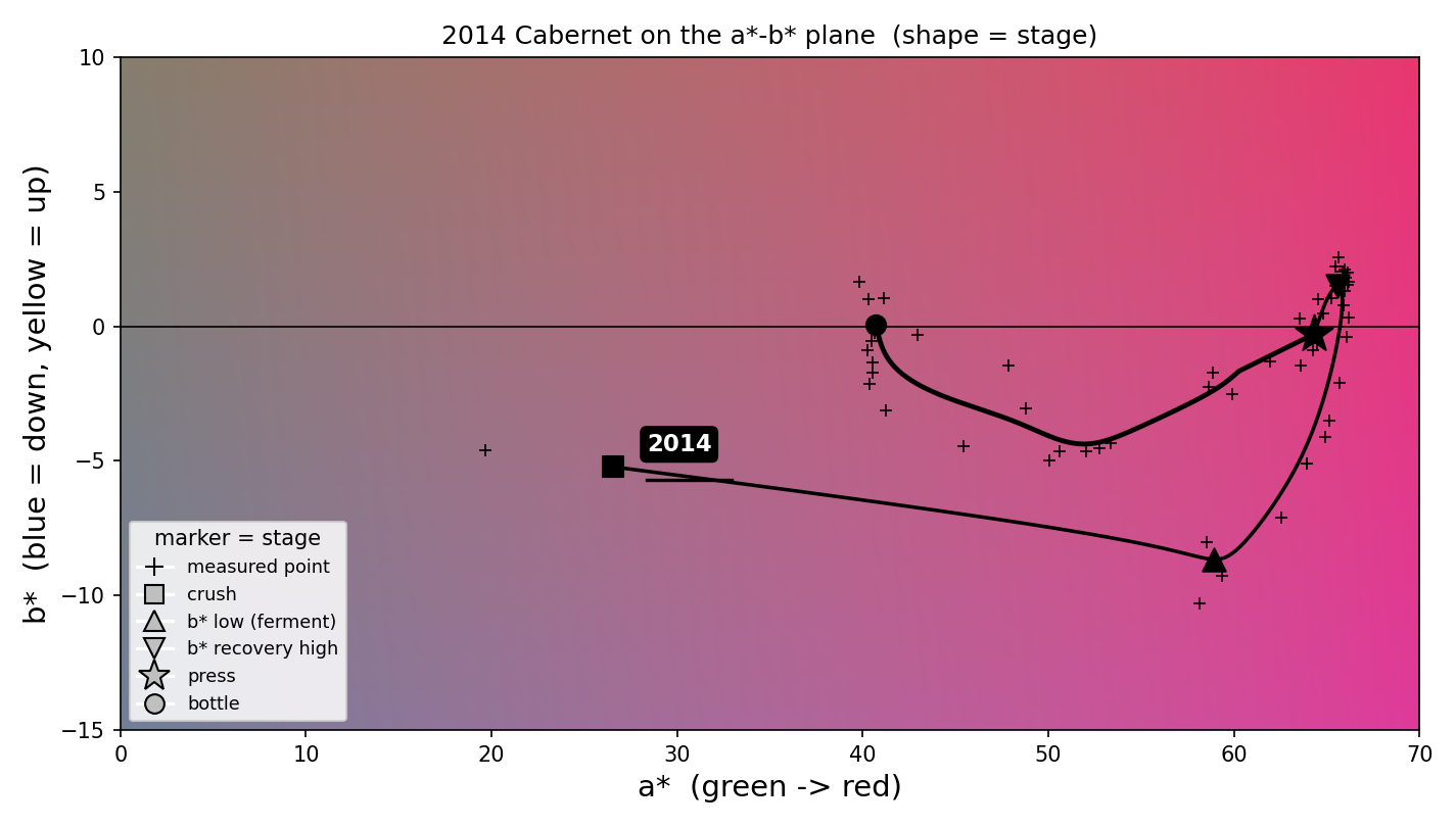
Figure 5. The 2014 Cabernet colour path, smoothed - fermentation lightly, aging more strongly - with the raw measurements shown as small crosses. The out-and-back loop and the slow inward drift toward brick are now legible. Square = crush, up/down triangles = the b* low and its recovery, star = press, dot = bottle.

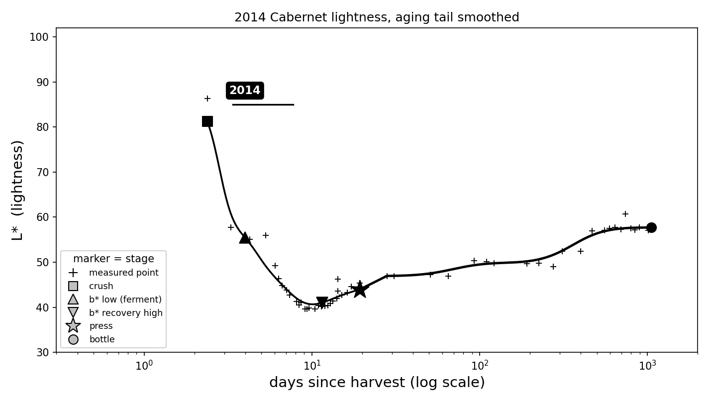
Figure 6. The 2014 Cabernet lightness, smoothed: a clean fermentation plunge to the press floor, then a gentle recovery in barrel. Raw measurements shown as crosses.

Five Vintages Compared

Now, let’s compare five Cabernet Sauvignon vintages. Each vintage is a black line with its own dash style and a distinct marker color; the marker shapes flag the stages (square = crush, up/down triangles = the b* low and recovery, star = press, dot = bottle). The 2017 wine is a blend cellar lot rather than a straight continuation of the single ferment we tracked, so its path across the press should be read with that caveat (marked *).

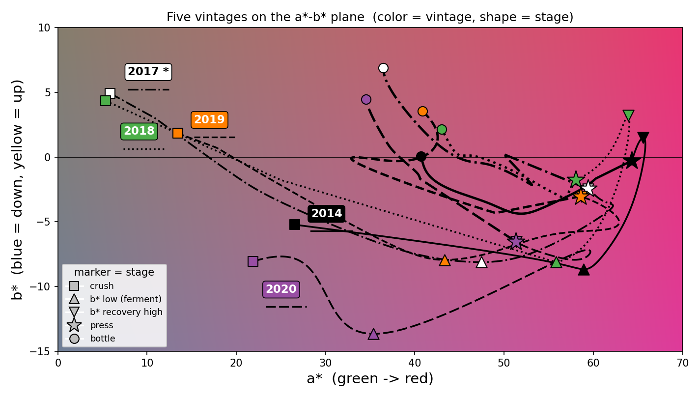
Figure 7. Five vintages on the a*-b* plane (b* axis -15 to +10). The background shows the colour of each a*-b* point; every vintage is a black line with its own dash style and a distinct marker colour, smoothed from crush to bottle. Shapes flag the stages: square = crush, up-triangle = b* low, down-triangle = recovery, star = press, dot = bottle. 2017 (marked *) is a blend cellar lot.

Lightness over time tells the complementary story: every vintage plunges to a similar dark floor by the press, then the smoothed tails fan out to different settled levels.

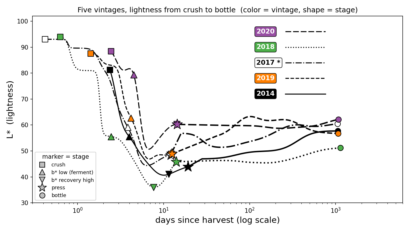
Figure 8. Five vintages, lightness L* from crush to bottle on a logarithmic time axis, smoothed. A shared fermentation plunge to the press floor (stars), then recovery to settled levels that track bottle age.

Table 2. Key CIE L*a*b* coordinates for the five vintages at five stages - fermentation start, the b* low point during fermentation, the subsequent b* recovery high, press, and bottling - arranged by stage so the vintages can be compared directly at each point. Values are read from the smoothed trajectories, so they match the markers in Figures 5-8. Time is days since harvest.

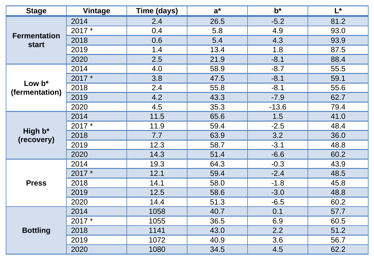
* 2017 is a blend cellar lot (see text). The high-b* row is the recovery peak reached after the purple low but before the press; for 2017, 2019, and 2020, this recovery is only partial (b* remains negative there), whereas 2014 and 2018 climb back into positive b*. 2020's fermentation start is taken from its first spectrum with measurable color (day 2.5); two earlier scans (days 0.4 and 1.4) had no visible absorbance - the near-colorless juice before extraction - and are excluded. Its b* minimum (day 4.5, L*~79) is still anomalously light relative to the other vintages.

What the Colors Tell Us

Color extraction is remarkably consistent across vintages, despite different growing seasons and evolving fermentation and cellaring protocols. Lightness falls rapidly after fermentation starts, b* values decrease (more blue) to a low before rising again, and a* values (redness) increase reaching a peak of 60-65 before press.
Aging is an orderly migration from purple toward brick. In the cellar, the color moves steadily inward and upward on the a*–b* plane: chroma fades as pigments polymerize and precipitate, and b* climbs across zero from the purple side to the brick side. This crossover is the single clearest marker of maturation, and it unfolds over years [5, 7].
Position along the aging tail tracks the purple-to-brick drift. Its extent, though, depends on vintage and barrel handling as much as on time: all five wines spent roughly three years in barrel, yet 2017 travels furthest into brick (highest b*) while 2014 stays closest to the purple side. Reading the end of each smoothed tail still gives a quick, quantitative sense of how far a wine has matured.
Lightness mirrors the color story. Each wine shows a sharp plunge in lightness as color builds during fermentation, a dark floor just before pressing, and a gradual recovery in the cellar. Fermentation drives color in and down; cellaring slowly lets it back out, shifting the hue.

Note that each cellar batch is followed only up to bottling — after bottling, the wine takes a new batch name and drops out of this dataset — so the tails end at or just before bottling rather than running on indefinitely. The five vintages together show a strikingly reproducible arc: consistent extraction to a common peak, then a slow drift from purple youth toward brick maturity whose extent is set as much by oak and vintage as by time. No great new revelations so far, still, there are significant differences between the vintages, which beg further questions

Where This Goes Next

A consistent color trajectory for every vintage opens several threads we mean to pull on:

Tie color to the underlying chemistry. The same spectra already yield phenolic estimates — free and total anthocyanins, tannins, polymeric pigment — so we can test how directly the a*/b* drift tracks the polymerization and precipitation that drive it.
Put a number on aging speed. Fit each smoothed tail with a single rate — for instance a hue half-life analogous to the color half-life we use for fermentation — so vintages can be ranked by how fast they brown, and relate that rate to cellar temperature and closure.
Predict from the early signal. Test whether the first weeks of extraction, or the color at press, foretell where a wine lands after a few years in the cellar.

• Link color to the kinetic fingerprint. Join these color trajectories to the fermentation fingerprints from the Modeling the Fermentation page.

References

[1] CIE (2004). Colorimetry, 3rd edition. CIE 15:2004. Vienna: Commission Internationale de l’Éclairage.

[2] OIV (2006). Determination of chromatic characteristics according to CIELab. Method OIV-MA-AS2-11, Compendium of International Methods of Analysis. Paris: Organisation Internationale de la Vigne et du Vin.

[3] Savitzky, A., & Golay, M. J. E. (1964). Smoothing and differentiation of data by simplified least squares procedures. Analytical Chemistry, 36(8), 1627–1639.

[4] Ribéreau-Gayon, P., Glories, Y., Maujean, A., & Dubourdieu, D. (2006). Handbook of Enology, Volume 2: The Chemistry of Wine Stabilization and Treatments (2nd ed.). Chichester: Wiley.

[5] Glories, Y. (1984). La couleur des vins rouges. Connaissance de la Vigne et du Vin, 18(3), 195–217 and 18(4), 253–271.

[6] Boulton, R. (2001). The copigmentation of anthocyanins and its role in the color of red wine: A critical review. American Journal of Enology and Viticulture, 52(2), 67–87.

[7] Pérez-Magariño, S., & González-San José, M. L. (2004). Evolution of flavanols, anthocyanins, and their derivatives during the aging of red wines. Journal of Agricultural and Food Chemistry, 52(5), 1181–1189.

Last revision: draft8 · July 12, 2026